The following instructions show how to use conditional formatting in Microsoft Excel to automatically highlight the current week, based on a column with a “Week Commencing” date (a Monday).
On this pageJump to a section
This allows you to visually show which row relates to the current week.
For this example, we will use the following data and assuming that the date is 19/05/2024 (19 May 2024).
Example Table Content
| Employee | Task | Week Commencing |
|---|---|---|
| John Doe | Project A | 15/05/2024 |
| Jane Smith | Project B | 22/05/2024 |
| Mark Brown | Project C | 29/05/2024 |
Steps
- Open Excel File
Open the Excel file with your data. - Select the Range
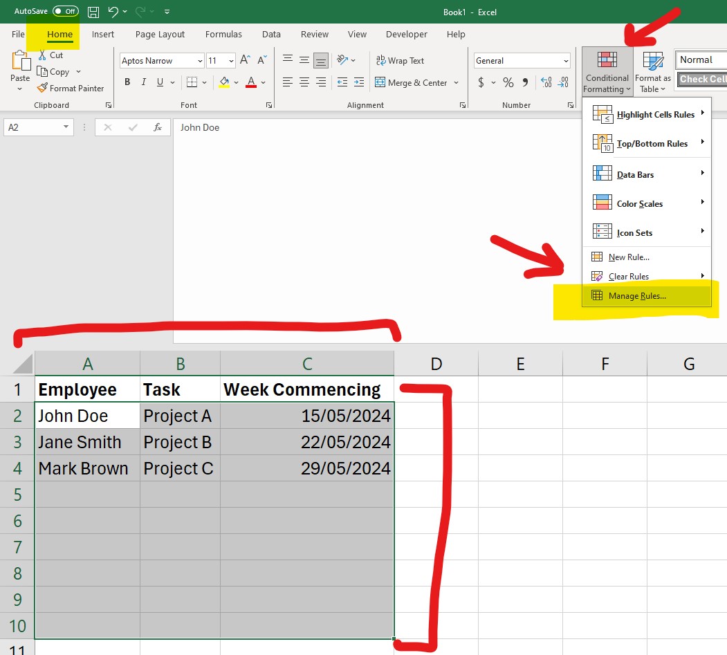
Select the range of rows you want to apply conditional formatting to (e.g., A2:C10). - Open Conditional Formatting
Go to the ‘Home’ tab, click on ‘Conditional Formatting’, then select ‘Manage Rules’.
Click on the ‘New Rule’ button - Use a Formula to Determine Which Cells to Format
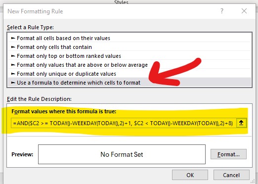
In the New Formatting Rule dialog, select ‘Use a formula to determine which cells to format’. - Enter the Formula
Enter the following formula:=AND($C2 >= TODAY()-WEEKDAY(TODAY(),2)+1, $C2 < TODAY()-WEEKDAY(TODAY(),2)+8)
- This formula calculates the start of the current week (Monday) and checks if the “Week Commencing” date falls within this week.
- Set the Format
Click Format, choose your desired formatting (e.g., fill colour), and click OK. - Apply the Rule
Click OK again to apply the rule.
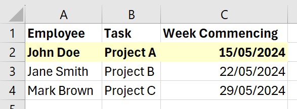
Your rows where the “Week Commencing” dates fall within the current week will now be highlighted.
Explanation of the Formula
- TODAY(): Returns today’s date.
- WEEKDAY(TODAY(), 2): Returns the day of the week (Monday = 1, …, Sunday = 7).
- TODAY() – WEEKDAY(TODAY(), 2) + 1: Calculates the most recent Monday.
- AND($C2 >= [Last Monday], $C2 < [Next Monday]): Checks if the date in column C is within the current week.