The following instructions show how to use conditional formatting in Microsoft Excel to automatically highlight the current week, based on a column with a “Week Commencing” date (a Monday).
This allows you to visually show which row relates to the current week.
For this example, we will use the following data and assuming that the date is 19/05/2024 (19 May 2024).
Example Table Content
| Employee | Task | Week Commencing |
|---|---|---|
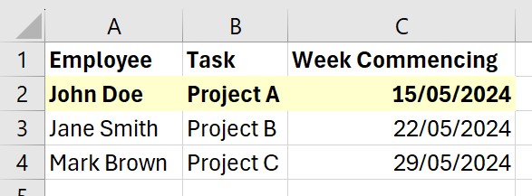
| John Doe | Project A | 15/05/2024 |
| Jane Smith | Project B | 22/05/2024 |
| Mark Brown | Project C | 29/05/2024 |
Steps
- Open Excel File
Open the Excel file with your data. - Select the Range
Select the range of rows you want to apply conditional formatting to (e.g., A2:C10). - Open Conditional Formatting
Go to the ‘Home’ tab, click on ‘Conditional Formatting’, then select ‘Manage Rules’.
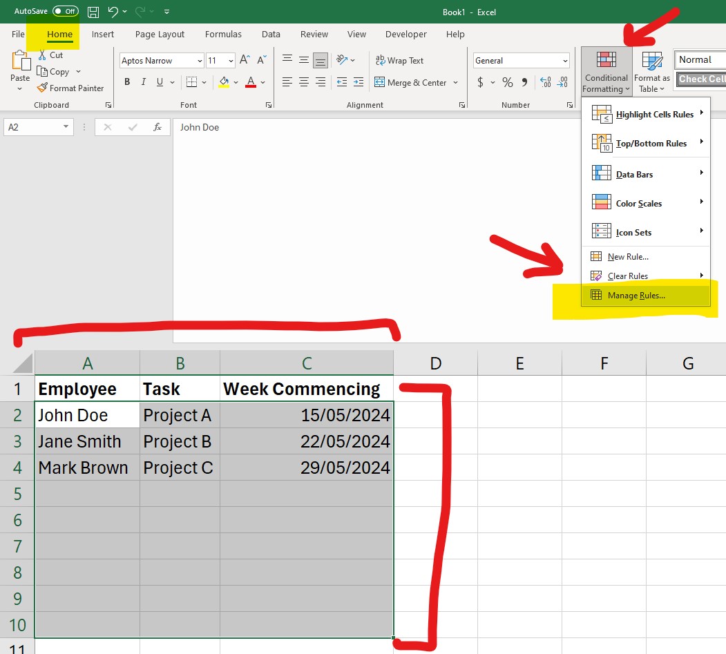
Click on the ‘New Rule’ button - Use a Formula to Determine Which Cells to Format
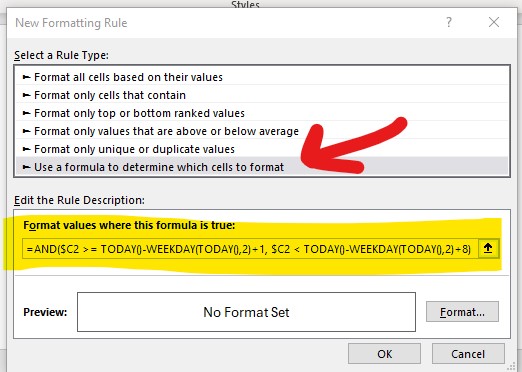
In the New Formatting Rule dialog, select ‘Use a formula to determine which cells to format’. - Enter the Formula
Enter the following formula:=AND($C2 >= TODAY()-WEEKDAY(TODAY(),2)+1, $C2 < TODAY()-WEEKDAY(TODAY(),2)+8)
- This formula calculates the start of the current week (Monday) and checks if the “Week Commencing” date falls within this week.

- Set the Format
Click Format, choose your desired formatting (e.g., fill colour), and click OK. - Apply the Rule
Click OK again to apply the rule.
Your rows where the “Week Commencing” dates fall within the current week will now be highlighted.
Explanation of the Formula
- TODAY(): Returns today’s date.
- WEEKDAY(TODAY(), 2): Returns the day of the week (Monday = 1, …, Sunday = 7).
- TODAY() – WEEKDAY(TODAY(), 2) + 1: Calculates the most recent Monday.
- AND($C2 >= [Last Monday], $C2 < [Next Monday]): Checks if the date in column C is within the current week.