The following steps show how to create a pivot table and chart that has two values (value and percent of total) but the chart only displays one value.
This process shows you how to hide values in the pivot chart.
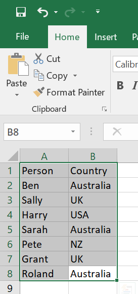
- Select the table you want to create the pivot chart from
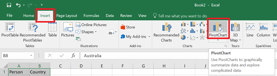
- Click on the ‘Insert’ ribbon menu
- Click on the ‘PivotChart’ button
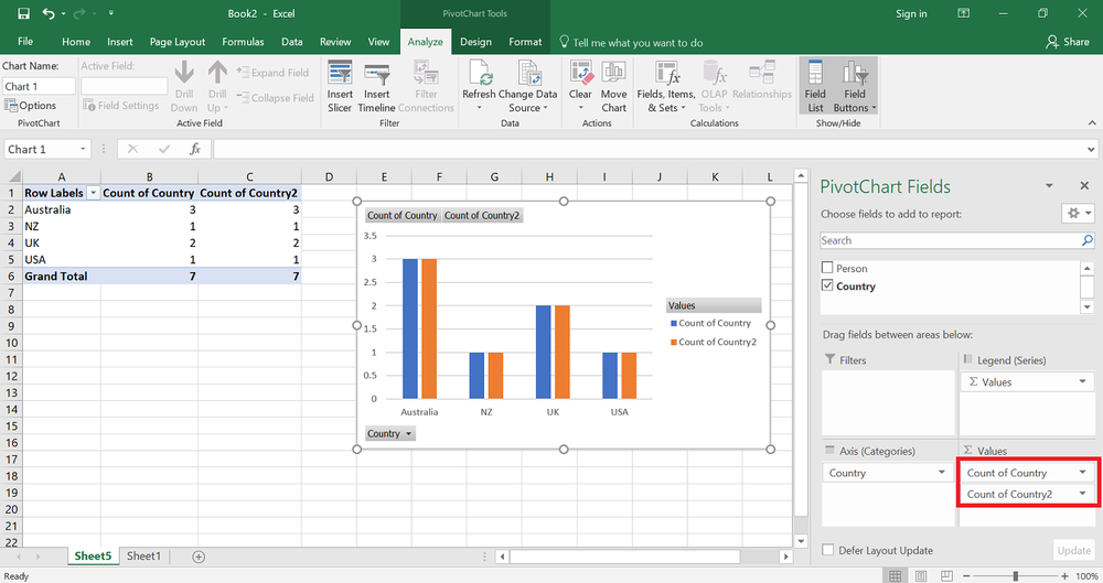
- Drag the value you want to chart TWICE into the ‘Values’ box
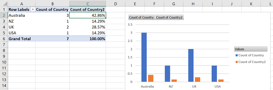
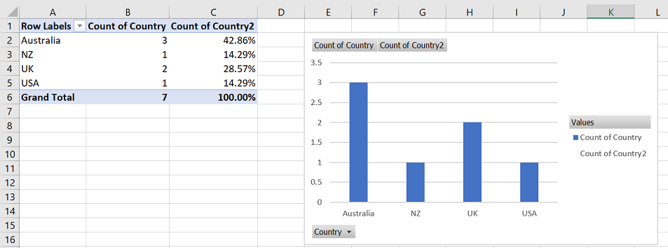
- The pivot table will now how the value shown twice
- Right-click on the second value in the pivot table and choose ‘Show Values As’ -> ‘% of Grand Total’
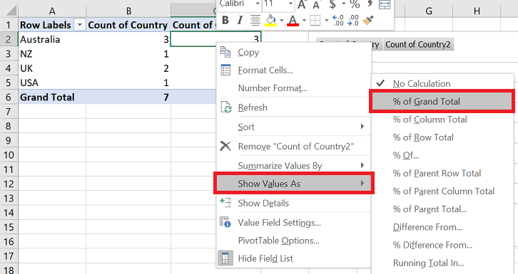
- The pivot chart will update
- Now we want to hide the percent value from the chart. Excel doesn’t offer an easy solution to this – instead we need to use the formatting to make the column hidden.
- Right-click on the column you want to hide and choose ‘Format Data Series’
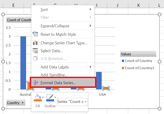
- The Format Data Series settings will appear at the right of the screen
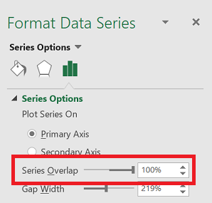
- On the ‘Series Options’ tab set ‘Series Overlap‘ to ‘100%’
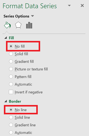
- Now open the ‘Fill & Line’ tab (paint bucket icon)
- Set ‘Fill’ to ‘No fill’
- Set ‘Border’ to ‘No line’
- The pivot chart will now only display one value – hiding the percentage of total value from the pivot table
Reference: https://superuser.com/questions/815798/have-pivot-chart-show-only-some-columns-in-pivot-table