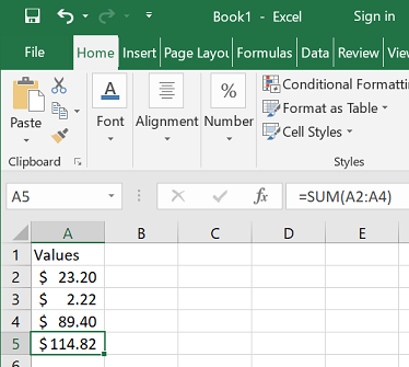
Cell references in Excel formulas typically use their position in the worksheet – e.g. A2 for a single cell or A2:A4 for a range.
But as formulas get more complicated this can lead to a confusing mess of letters and numbers.
The answer – named cell references.
With named cell references you can use words to refer to cells – e.g. total for a single cell or values for a range.
So how do you do it?
If we had a formula like below:
=SUM(A2:A4)
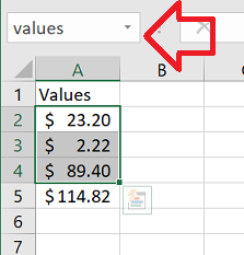
To create a named cell reference you simply select the cell or the range and enter type the name into the box above the worksheet.
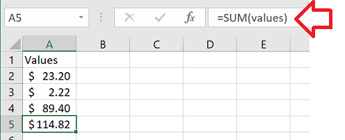
Now you can refer to the same range using the name, e.g.
=SUM(values)
But wait, there are limits !
- First character must be a letter, underscore (_) or backslash (/)
- Can only use letters, numbers, periods (.) and underscores (_)
- Name length maximum is 255 chracters
- Names are not case sensitive – you can use upper and lowercase, e.g. Total_Price – but Excel considers it the same as total_price, TOTAL_PRICE etc.
- Can’t use ‘C’, ‘c’, ‘R’ and ‘r’ – these are reserved terms for shorthand references
- Can’t make names that are the same as a typical cell reference – e.g. A2:A4 or A2
- Can’t use spaces – periods (.) and undersores (_) can be used to separate words, e.g. total_price
Reference: