The following guide shows four different ways to insert tick and cross symbols in Excel documents.
Ticks and cross symbols are useful visual cues in a dataset, typically representing “yes/no” or “true/false” values.
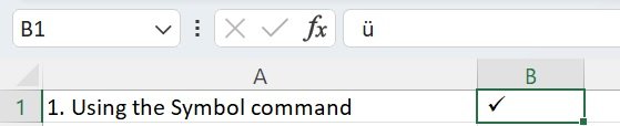
1. Using the Symbol command:
- Select the cell where you want to insert a checkmark.
- Navigate to the
Inserttab >Symbolsgroup, and click onSymbol. 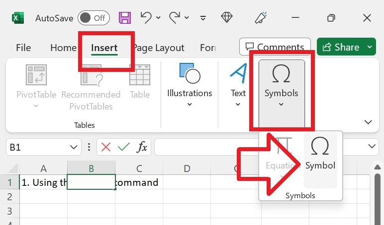
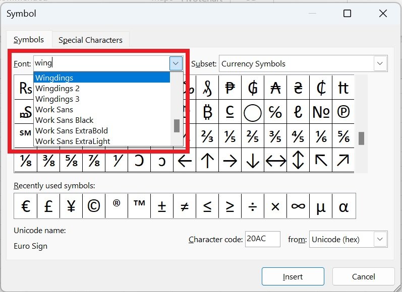
- In the
Symboldialog box, on theSymbolstab, click the drop-down arrow next to theFontbox, and selectWingdings. 
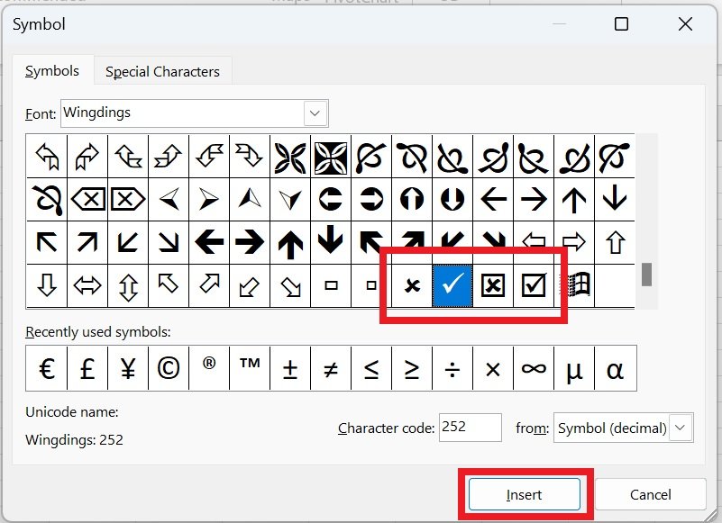
- A couple of checkmark and cross symbols can be found at the bottom of the list. Select your preferred symbol, and click
Insert. 
- Finally, click
Closeto close theSymbolwindow. 
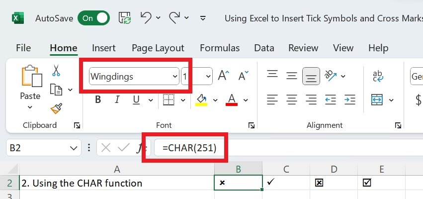
2. Using the CHAR function:
This method works best for inserting a tick in an empty cell.
- Enter the formula for the desired symbol
- checkmarks are
=CHAR(252)or=CHAR(254) - cross symbol are
=CHAR(251)or=CHAR(253)
- checkmarks are
- Apply the
Wingdingsfont to the cell 
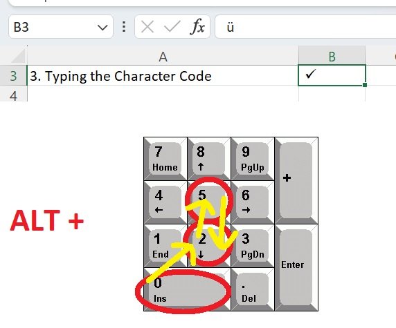
3. Typing the Character Code:
- Select the cell where you want to put a tick.
- Change the cell font to
Wingdings - On your keyboard, press and hold ALT while typing one of the following character codes on the numeric keypad:
- Alt+0252 for a tick,
- Alt+0254 for a tick in a box,
- Alt+0251 for a cross, or
- Alt+0253 for a cross in a box.

4. Inserting Tick Symbol as an Image:
- If you want to use a specific tick symbol – you can copy an image into your Excel document.
- For example:
- Tick:

- Cross:

- Tick: