The steps below detail how to take a column of values, some that are duplicates, and to list the unique values. There are two ways this can be done – replacing the existing column or creating a new column.
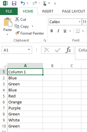
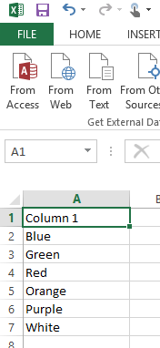
For example, our column looks like this:
Method 1: replace the current column
- Select the column of data
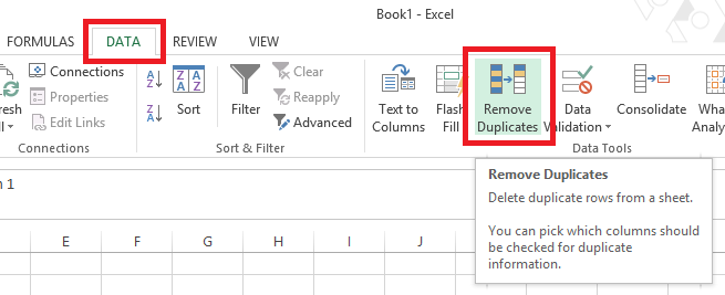
- Open the ‘DATA’ ribbon
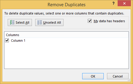
- Click on the ‘Remove Duplicates’ button

- If your column has a header, click the ‘My data has headers’ tick box
- Click ‘OK’

- The original column will now be replace with only the unique values

Method 2: create a new column
- Select the column of data
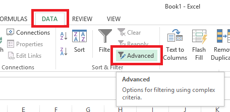
- Open the ‘DATA’ ribbon

- Select ‘Copy to another location’
- Make sure that ‘List range’ and ‘Criteria range’ has the same value – if it doesn’t, copy the range from ‘List range’ to ‘Criteria range’
- Use the button next to the ‘Copy to’ field to select where to copy the unique values to
- Place a tick next to ‘Unique records only’
- Click ‘OK’

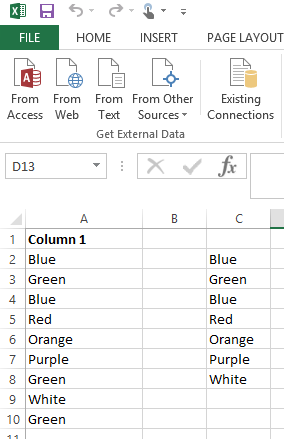
- You will now have a new list of unique values.