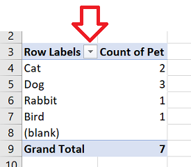
If you need to create a pivot table chart on a range that includes blank rows you’ll end up with a (blank) label.
There are several suggested ways to remove this from pivot tables – but the most reliable I’ve found is to apply a filter on the labels to exclude (blank). The filter will stay applied even when the data is refreshed – automatically excluding (blank).
The steps below show how I do this.
How to filter pivot table columns by label
- In your pivot table, click on the down down button next to ‘Row Labels’
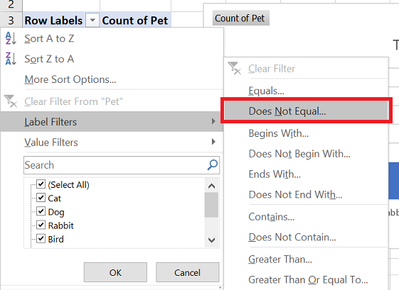
- Click on ‘Label Filters’ -> ‘Does Not Equal’
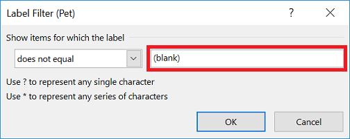
- Enter (blank) in the box and click ‘OK’
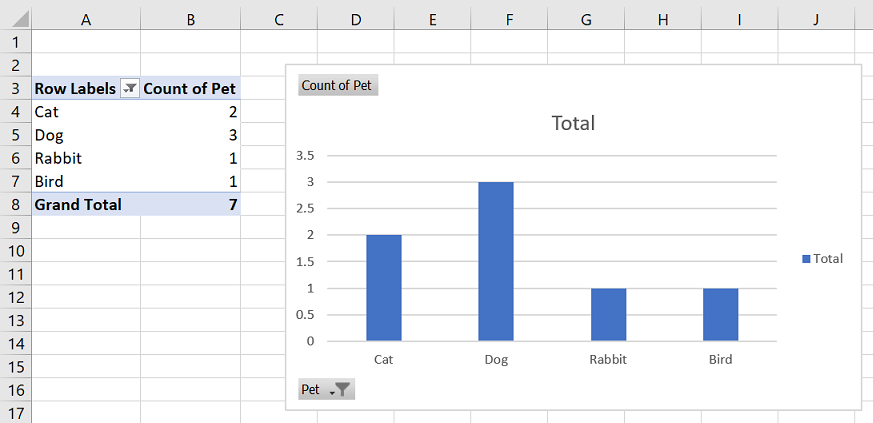
- The (blank) items will now automatically be excluded from the pivot table and pivot table chart.
Reference:
That option is greyed out 🙁
Thanks a lot! It helped me out big time!
This works BUT: I want to create a (top 10) AND (exclude blanks). You can’t select both at the same time in the filters. Any way to do this without deselecting the blank option in the filters? I can’t do this anyway if source data is empty as it automatically ‘selects all’. Any other way to exclude blanks?
Go to the pivot table options and select from the totals & filters tab the “allow multiple filters per field” option. Then you can do both 😉
Hi
This works but I want to create a table with:
a) top 10
b) does not contain blanks
by this way I can only choose either.
Any way to do both? (not by deselecting the blank)
Hello there Adrian…. That post a very valuable piece of info. Love you….
Hello my loved one! I want to say that this post is awesome, great written and include almost all vital infos. I’d like to see extra posts like this.
This is very helpful… thank u