Excel 2016 – How to filter pivot table data

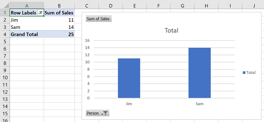
The steps below will show how to hide data from a pivot table based on the value.

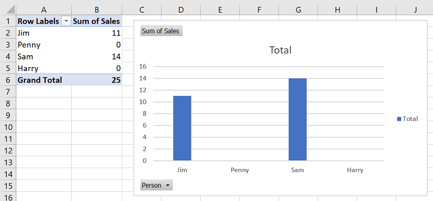
In this example we’ll be hiding data where the value is 0. In this case, both Penny and Harry will be excluded from the pivot table chart.

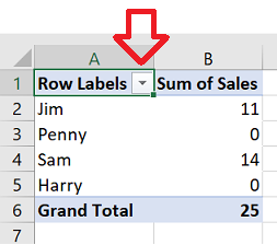
1. In your pivot table, click on the down down button next to ‘Row Labels’
2. 
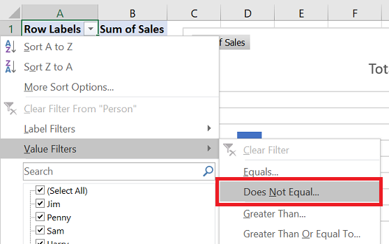
3. Click on ‘Value Filters’ -> ‘Does Not Equal’
4. 
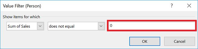
5. Enter 0 in the box and click ‘OK’
6. 
7. The data with a 0 value will now be automatically excluded – even when the pivot table is refreshed.
8. 

 

Reference: https://www.extendoffice.com/documents/excel/1876-excel-pivot-table-hide-zero-values.html